| T h e P a n g e a M o d e l |
 |
| T h e P a n g e a M o d e l |
|
| > Description > Extended | [login] |
This section provides an extended introduction/description about the main mechnisms invovled in Pangea.
The general flow of operations in Pangea is represented in Fig.1. We start with non-gridded geo-referenced data that characterize the natural system (loosely defined as "the world"). Using its GIS engine [1], Pangea builds a set of grids that cover all relevant media, hence defining the geometrical system, and projects geo-referenced data in this system. Gridded data and geometric and topological parameters are then re-indexed [2] into a mathematical compartmental system called virtual system. This system is solved [3] (for e.g. environmental concentrations at steady-state), further computations are performed (e.g. population exposure), and the solution is projected back onto relevant grids [4] for analysis/visualization.
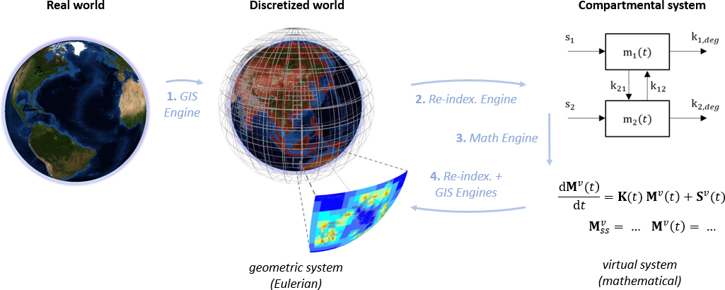
Figure 1 - General flow of operations in Pangea.
Goverining equations are simples; the virtual system is a linear system of first order ordinary differential equations (with time-dependent or constant coefficients) of dimension \(n^v\) :
\[\frac{\mathrm{d}m(t)}{dt} = \mathbf{K}(t)\:m(t) + s(t) \quad \text{or as simple as} \quad \frac{\mathrm{d}m(t)}{dt} = \mathbf{K}\:m(t) + s\] where \(m(t)\in\mathbb{M}_{n^v \times 1}\) is a vector of masses of pollutant, \(s(t)\in\mathbb{M}_{n^v \times 1}\) is a vector of emissions, and \(\mathbf{K(t)}\in\mathbb{M}_{n^v \times n^v}\) is a matrix of transfer rate coefficients.
The complexity lies in the construction of this system: how to go from a set of geo-referenced data to a global system of 3D multi-scale grids covering all relevant media and whose cells delineate inhomogeneous content (e.g. terrestrial grid cells contain all relevant terrestrial media), and then to a mathematical compartmental system the describes the evolution of a set of homogeneous compartments.
The model structure (functional blocks) is represented in Fig.2. While Pangea v1 was about half MATLAB and half Python/ArcGIS, the mid-term goal with v2 is to propose a MATLAB only model. The main reason is that it is difficult to maintain a model that invloves multiple language, and difficult for users to understand what must be done, when and where. Version 1 was therefore difficult to analyze and debug for both developers and users. Fig.2 shows a Core, a re-indexing engine, a computation engine, a set of environmental models, a GIS engine, and a set of more general models (atmospheric, hydrological, etc). While this figure is a bit outdatted (the model was recently restructured), it shows most constitutive blocks of the model.
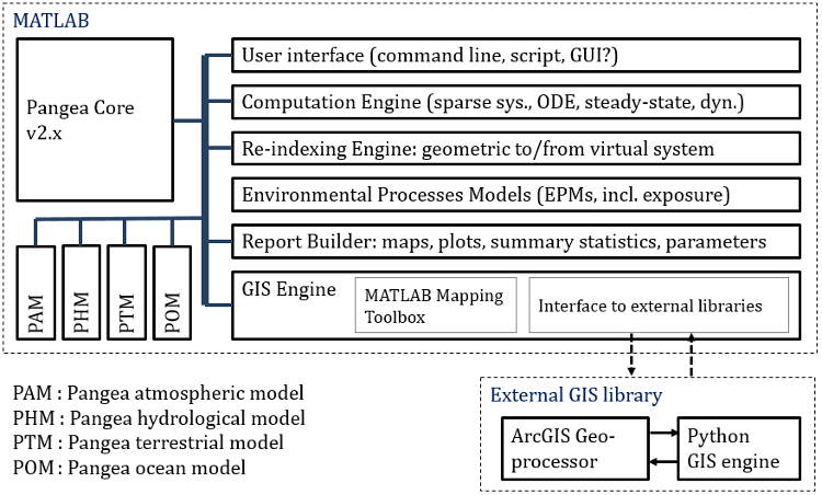
Figure 2 - Model structure.
In practice, Pangea comes as a bundle with:
The core of the model is a MATLAB package named Pangea (folder [pangea-root]/Model/[version,revision]/+Pangea). A project is a MATLAB M-Files which builds an instance of the Pangea.Model class and performs a series of operations for setting up all relevant components of the project. Multiple approaches are possible, ranging from the creation of a pre-defined type of "easy" project (e.g. single point source with default parameters) such as below:
% - Initialize and load model.
addpath( '..\..\Model\Current' )
model = Pangea.Model()

% - Create point source ezProject, add pollutant and source.
% Source @ lon = 4, lat = 49, alt = 10m, to air, intensity = 1EMU/day.
project   = model.addEzProject( 'PointSource' ) ;
pollutant = project.addPollutant( '71-43-2', 'Benzene' ) ;
project.addPointSource( 4, 49, 10, 'air', pollutant, 1 ) ;

% - Run and export.
project.run() ;
project.results.export() ;
.. to M-Files that contain several hundreds of lines for defining specifically every relevant parameter.
Pangea comes with a default set of grids and media. Grids are built at runtime and hence project-specific. This allows advanced users to build their own grids. The set of media is intimately bound to the set of EPMs; yet, advanced users can introduce new media if they provide the EPMs that describe/model pollutant fate and transport with these media and between these media and other media.
| Background grid | : | single layer, low resolution, e.g. 40x20 cells over whole world. |
| Results grid | : | single layer, multi-scale; this is the grid onto which are projected all the results ultimately. |
| Atmospheric grid | : | 17 layers, 3D multi-scale. |
| Terrestrial grid | : | single layer, clustered, weakly multi-scale. |
| Sediments grid | : | piggy-back of terrestrial grid, limited to cells which contain fresh water. |
| Sea/ocean grid | : | single cell, more complex version under dev. (with very priority), complexity comes from coastal zones. |
| Air | : | ... |
| Fresh water | : | ... |
| Sediments | : | ... |
| Natural lands | : | ... |
| Agricultural lands | : | ... |
| Sea water | : | ... |
The refinement potential (RP) is a practical solution for specifying constraints on the resolution, as a basis for building multi-scale grids. It is by definition a global scalar field whose value in each point of the globe defines the user "interest for high resolution". In practice, it is a raster that results from multiple, weighted contributions, e.g.: population density, distance from source(s), etc.
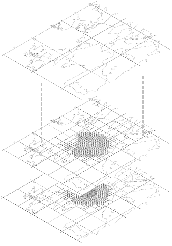
Fig.3 provides an example. A background grid with low resolution is represented on the left. The center respresents a RP obtained as a weighted sum between components made of a raster of population counts, a step function of the distance from a source that is a the center of the disks, and a flag " in land". The figure on the right is the refined multi-scale grid obtained after an iterative refinement procedure.
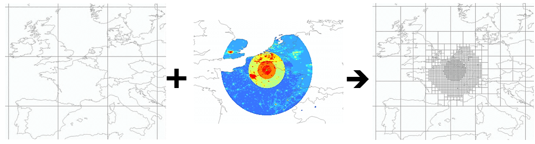
Figure 3 - Background grid and refinement potential; resulting multi-scale grid.
The iterative procedure is depicted in another context (RP = global raster of population counts) in Fig.4 : depth 0 is the background grid; the potential is integrated on this grid (providing a summary (SUM of pixels in practice) per cell), and all cells whose summary value is above a user-defined threshold are refined (e.g. split in 4). This defines a new grid; the potential is integrated over this new grid, and so on..
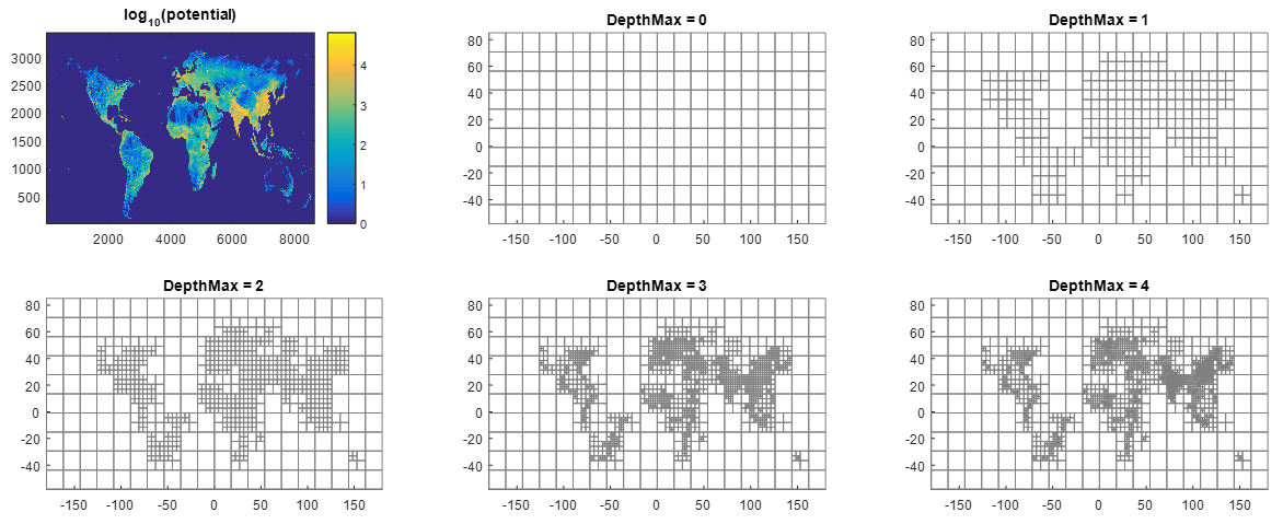
Figure 4 - Refinement steps.
The Background grid is a user-defined regular/rectangular grid in the space of longitudes and latitudes that covers the globe (e.g. 40x20 cells). It is the starting point of the refinement procedure.
The Results grid is a multi-scale grid obtained through the refinement procedure explained above, which is the grid onto which all results are projected ultimately. It is user-defined and project specific, built with a high resolution as specified by user through the definition of the refinement potential and low(er) resolution elsewhere. Pangea uses this grid (as well as all intermediary grids obtained during the refinement procedure) e.g. in its procedure for buildinging the default atmospheric grid, where it defines the first atmospheric layer. Projecting all results onto this grid at the end is required for comparison: environmental concentrations of pollutant in the air and in fresh water could not be compared if they were expressed on different geometries.
|
The default atmospheric grid is made of 17 layers based on grids obtained during the refinement process described in the previous section. The first layer is the Results grid. The second layer is the grid defined at the last intermediary step of the refinement, and so on until we reach the background grid. All layers above are then defined using the background grid. In Pangea v1.x, layers' altitudes where defined to match GEOS-Chem sigma surfaces. Pangea v2 currently implements (as a prototype) an atmospheric model which interpolates in 3D, making it possible to specify user-defined altitudes. |
|
Figure 5 - Atmospheric grid/layers. |
The default terrestrial grid is based on the WWDRII 0.5°\(\times\)0.5° fresh water model. A new version (in development) is based on the HydroBASINS model/database, and will be available sometime in 2016. In any case, the hydrology defines the terrestrial grid geometry of watersheds.
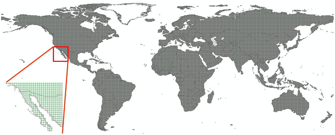
Figure 6 - WWDRII 0.5°\(\times\)0.5° fresh water model grid (with a few modifications (cleaning)).
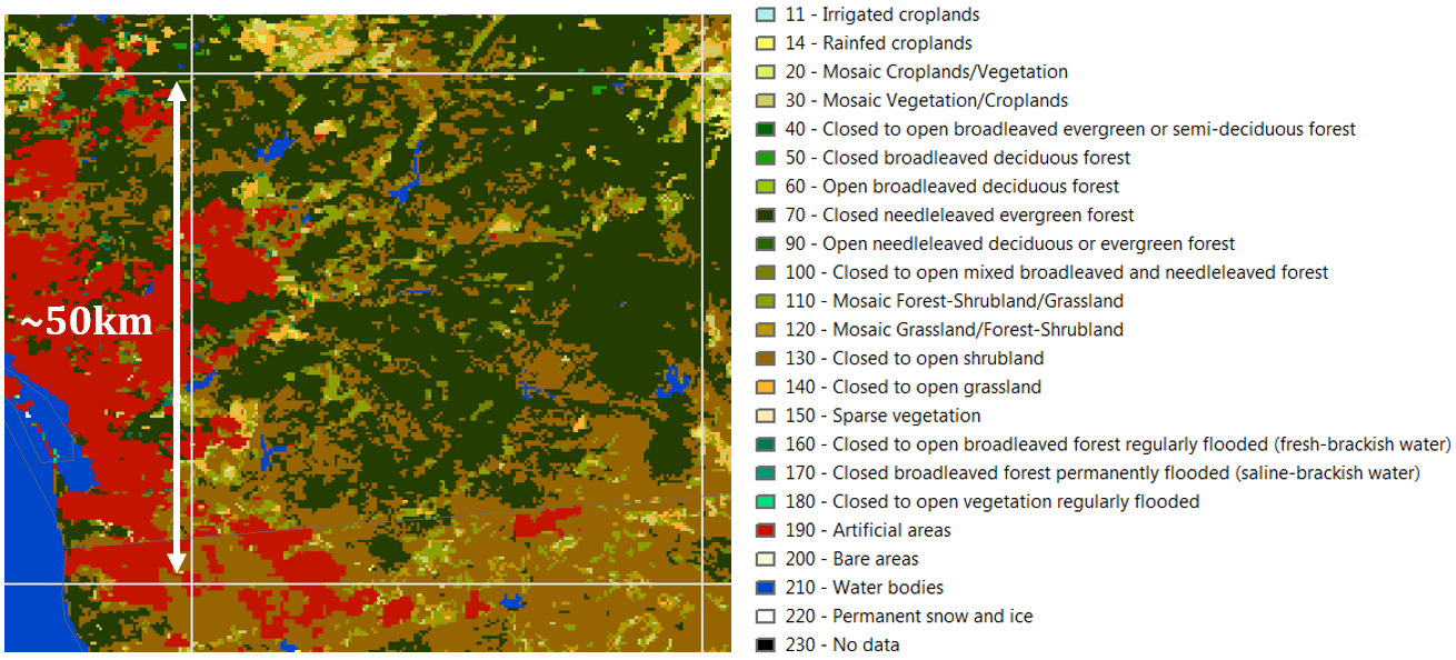
Figure 7 - Land cover types as defined by GlobCover. The white cell represents approximately the size of a cell from the WWDRII native grid.
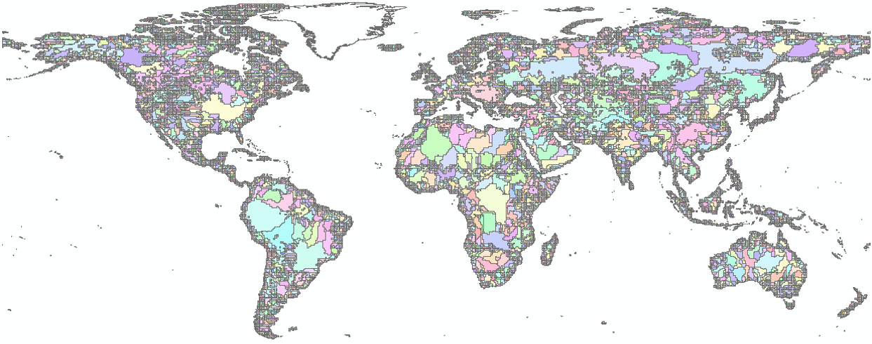
Figure 8 - Clustered terrestrial grid.
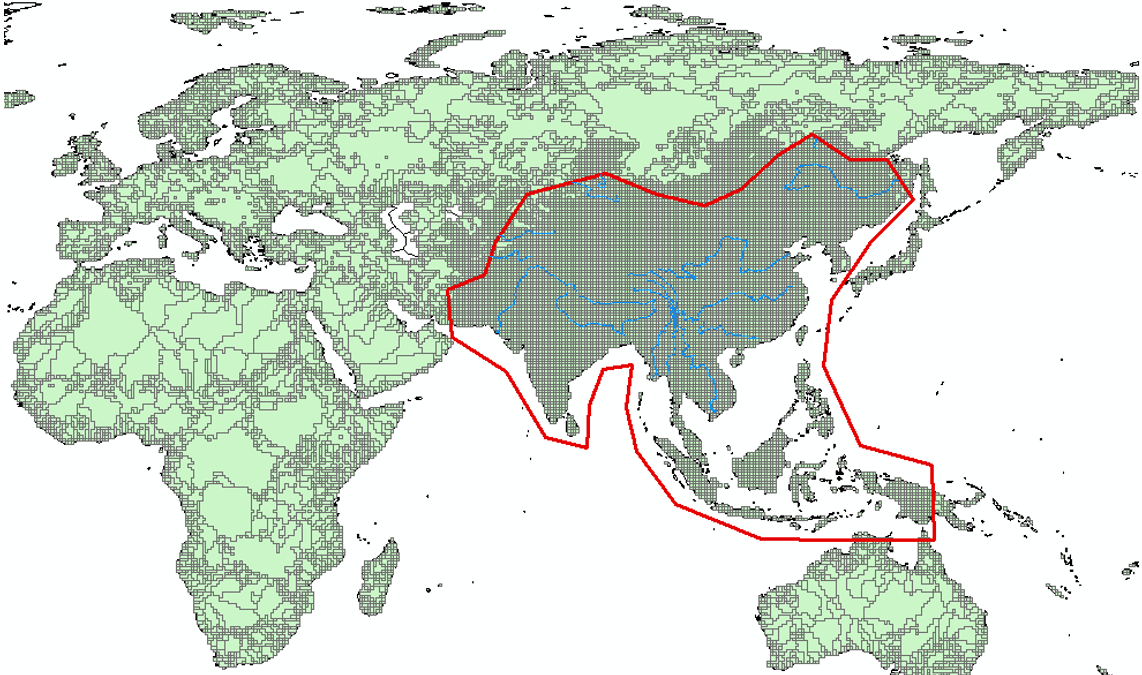
Figure 9 - Clustered terrestrial grid, unclustered over a region of interest.
The sediments grid is a piggy-back of the terrestrial grid, reduced to cells with a non-null fresh water content.